
Spectral Clustering From Scratch
In this blog post, we will be creating a simple version of the Spectral Clustering algorithm using Python.
What is Clustering?
Clustering refers to the task of separating a data set into a certain number of groups based on similarity between data points. K-means is perhaps the most common way to achieve this task which uses a distance metric relative to a centroid to cluster data.
We will be using Spectral Clustering which looks at data points in the data as a connected graph and then partitions the graph into subgraphs i.e the clusters. This method is more suited for data which is shaped ‘weird’ as shown below:
# import these packages
import numpy as np
from sklearn import datasets
from sklearn.cluster import KMeans
from matplotlib import pyplot as plt
-
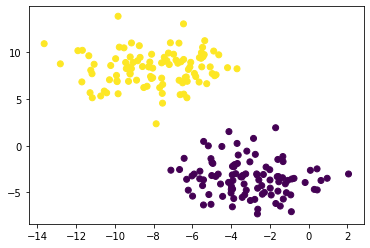
A simple clustering problem
n = 200
np.random.seed(1111)
X, y = datasets.make_blobs(n_samples=n, shuffle=True, random_state=None, centers = 2, cluster_std = 2.0)

km = KMeans(n_clusters = 2)
km.fit(X)

plt.scatter(X[:,0], X[:,1], c = km.predict(X))
-
datasets.make_blogs(): This function creates a dataset of clusters based several parameters. It returns:- X : a \(\mathbf{R}^{n \hspace{0.08cm} x \hspace{0.08cm} 2}\) array representing points in the
2Dplane - y : the true cluster labels for each point in X
- X : a \(\mathbf{R}^{n \hspace{0.08cm} x \hspace{0.08cm} 2}\) array representing points in the
KMeans(): creates a k-means clustering model
-
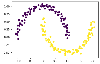
A complex clustering problem
np.random.seed(1234)
n = 200

X,y = datasets.make_moons(n_samples=n, shuffle=True, noise=0.05, random_state=None)

km = KMeans(n_clusters = 2)
km.fit(X)
plt.scatter(X[:,0], X[:,1], c = km.predict(X))

We can see that our KMeans Clustering does not do justice to these crescent shaped clusters in our data. This is because k-means, by design, looks for circular clusters in the data.
Let’s see if Spectral Clustering does a better job!
About Notation
In all the math below:
- Boldface capital letters like \(\mathbf{A}\) refer to matrices (2d arrays of numbers).
- Boldface lowercase letters like \(\mathbf{v}\) refer to vectors (1d arrays of numbers).
- \(\mathbf{A}\mathbf{B}\) refers to a matrix-matrix product (
A@B). \(\mathbf{A}\mathbf{v}\) refers to a matrix-vector product (A@v).
Breaking the Algorithm Step by Step
Step 1: Create the Similarity Matrix
-
The
Similarity Matrix\(\mathbf{A}\) should be a matrix (2dnp.ndarray) with shape(n, n)wherenis the number of data points. -
An entry in \(\mathbf{A}\) represented by
A[i,j]is the distance between pointiandj. Thus,A[i,i], the diagonal entries, should be 0 because the distance between a point and itself is 0. -
When constructing \(\mathbf{A}\), we use a parameter
epsilon. EntryA[i,j]of the matrix ‘A’ should be equal to1ifX[i](the coordinates of data pointi) is withinepsilondistance ofX[j](the coordinates of data pointj). Else,A[i,j]should be 0.
def similarity_matrix(X, epsilon):

    # construct the pairwise distance matrix
    A = sklearn.metrics.pairwise_distances(X, metric='euclidean')

    # make the entries 1 or 0 if the condition is satisfied
    A[A < epsilon] = 1
    A[A != 1] = 0

    np.fill_diagonal(A,0) # make all diagonal entries 0

    return A

A = similarity_matrix(X, 0.4)
A
array([[0., 0., 0., ..., 0., 0., 0.],
       [0., 0., 0., ..., 0., 0., 0.],
       [0., 0., 0., ..., 0., 0., 0.],
       ...,
       [0., 0., 0., ..., 0., 0., 1.],
       [0., 0., 0., ..., 0., 0., 0.],
       [0., 0., 0., ..., 1., 0., 0.]])
        0.        ]])
Step 2: Calculating Binary Norm Cut Objective
The matrix \(\mathbf{A}\) now contains information about each points and how near (within distance epsilon) it is to each other point. We now have to cluster the data points in X by partitioning the rows and columns of \(\mathbf{A}\).
Important Variables:
-
Let’s assume we have two clusters in our data: \(C_0\) and \(C_1\). We can say that every data point in \(\mathbf{X}\) is either in \(C_0\) or \(C_1\).
-
Let \(d_i = \sum_{j = 1}^n a_{ij}\). Thus, \(d_i\) represents the sum of each row of \(\mathbf{A}\).
-
Let
ybe the vector of cluster labels where \(y[i]\) is the cluster label (0 or 1) of pointiin \(\mathbf{X}\)
The Binary Norm Cut Objective:
The binary norm cut objective of a matrix \(\mathbf{A}\) is the function:
\[N_{\mathbf{A}}(C_0, C_1)\equiv \mathbf{cut}(C_0, C_1)\left(\frac{1}{\mathbf{vol}(C_0)} + \frac{1}{\mathbf{vol}(C_1)}\right)\;.\]In this expression,
- \(\mathbf{cut}(C_0, C_1) \equiv \sum_{i \in C_0, j \in C_1} a_{ij}\) is the cut of the clusters \(C_0\) and \(C_1\).
Ideally, we want \(\mathbf{cut}(C_0, C_1)\) to be 0 which would mean that the points in one cluster are seperated from the other cluster at distance greater than epsilon.
- \(\mathbf{vol}(C_0) \equiv \sum_{i \in C_0}d_i\), where \(d_i = \sum_{j = 1}^n a_{ij}\)
The volume of cluster \(C_0\) is a measure of the size of the cluster.
def cut(A,y):

    cut = 0
    c1_idx = np.where(y == 0)[0] # the points in cluster 1
    c2_idx = np.where(y == 1)[0] # the points in cluster 2

    for row in c1_idx:
        for col in c2_idx:
            cut += A[row,col]    # add the distance between points in the 2 clusters

    return cut
We can test cut of our points (with two clusters, see the figure) against randomly generated points.
We will notice that the cut for the true clusters is much smaller than the cut for the random clusters.
true_cut = cut(A,y) # the true cut

random_y = np.random.randint(2, size = 200) # create two random clusters
random_cut = cut(A,random_y) # the random cut

print(f"Cut for true labels: {true_cut} \nCut for random labels: {random_cut}")
Cut for true labels: 0.0
Cut for random labels: 397.0
Our assumption holds true. Moreover, notice that the cut for the true labels is 0; this means that for the given epsilon = 0.4 the points in the data can be clustered perfectly into two.
# computing the volumes
def vols(A,y):

    c1_idx = np.where(y == 0)[0] # points in C_0

    c2_idx = np.where(y == 1)[0] # points in C_1

    c1 = A[c1_idx,:]
    c2 = A[c2_idx,:]

    vol0 = np.sum(np.sum(c1, axis = 1)) # vol_C0
    vol1 = np.sum(np.sum(c2, axis = 1)) # vol_C1

    return tuple([vol0,vol1])

# computing the binary norm cut objective
def normcut(A,y):

    vol0 = vols(A,y)[0]
    vol1 = vols(A,y)[1]
    normcut = cut(A,y) * (1/vol0 + 1/vol1)
    return normcut
Now, let’s compare the normcut objective using both the true labels y and the fake labels we generated above.
print(f"Normcut for true labels: {normcut(A,y)} \nNormcut for random labels: {normcut(A,random_y)}")
Normcut for true labels: 0.0
Normcut for random labels: 1.0462545950710016
We want the binary normcut objective to be as small as possible which would mean:
-
There are relatively small number of points that overlap between the two clusters.
-
Neither \(C_0\) and \(C_1\) are too small i.e. their volumes are not small.
Time for some Quick Math
We have defined the binary normcut objective function which is minimized when the input clusters:
-
(a) Have small number of points that overlap between them.
-
(b) Aren’t too small i.e. the cluster volumes are not small.
Our objective is to minimize the binary normcut objective.
One mathematical approach is to find a vector y (that represents cluster labels for each point) such that normcut(A,y) is small.
However, this is an incredibly time-consuming optimization problem. The solution to this problem cannot be obtained in a time-efficient manner even with small number of points in the data.
Thus, we need a math trick here.
Here’s the trick: define a new vector \(\mathbf{z} \in \mathbb{R}^n\) such that:
\[z_i = \begin{cases} \frac{1}{\mathbf{vol}(C_0)} &\quad \text{if } y_i = 0 \\ -\frac{1}{\mathbf{vol}(C_1)} &\quad \text{if } y_i = 1 \\ \end{cases}\]Note that the signs of the elements of \(\mathbf{z}\) contain all the information from \(\mathbf{y}\): if \(i\) is in cluster \(C_0\), then \(y_i = 0\) and \(z_i > 0\).
In this way, the information about the cluster label of each point is preserved.
Also, this holds true:
\[\mathbf{N}_{\mathbf{A}}(C_0, C_1) = 2\frac{\mathbf{z}^T (\mathbf{D} - \mathbf{A})\mathbf{z}}{\mathbf{z}^T\mathbf{D}\mathbf{z}}\;,\]where \(\mathbf{D}\) is the diagonal matrix with nonzero entries \(d_{ii} = d_i\), and where \(d_i = \sum_{j = 1}^n a_i\) is the degree (row-sum) from before.
TO DO:
We will write a function called transform(A,y) to compute the appropriate \(\mathbf{z}\) vector given A and y using the formula above.
# 1
def transform(A,y):

    z = np.zeros(y.shape[0])                   # create an empty array
    z[np.where(y == 0)[0]] = 1/vols(A,y)[0]    # populate these indices with C_0 vol
    z[np.where(y == 1)[0]] = (-1)/vols(A,y)[1] # populate these indices with C_1 vol

    return z
# 2
z = transform(A,y)      # make the z vector
D = np.zeros((n, n))    # diagonal matrix D
d = np.sum(A, axis = 1) # vector of row-sums

np.fill_diagonal(D, d)  # fill the diagonal entries of D with d

a = 2*(z.T @ (D - A) @ z)/(z.T @ D @ z)
print(a)
print(normcut(A,y))
2.412442057241412
1.5875649591888283
-
This means our new function is an approximation of the
binary norm cut objective. -
Thus, optimizing this function will give us the approximate optimal solution of the
binary norm cut objectiveitself.
Step 3: Optimization
Now, we need to minimize:
\[R_\mathbf{A}(\mathbf{z})\equiv \frac{\mathbf{z}^T (\mathbf{D} - \mathbf{A})\mathbf{z}}{\mathbf{z}^T\mathbf{D}\mathbf{z}}\]subject to the condition \(\mathbf{z}^T\mathbf{D}\mathbb{1} = 0\).
We will use the minimize function from scipy.optimize to minimize the function orth_obj with respect to \(\mathbf{z}\).
def orth(u, v):
    return (u @ v) / (v @ v) * v

e = np.ones(n)

d = D @ e

def orth_obj(z):
    z_o = z - orth(z, d)
    return (z_o @ (D - A) @ z_o)/(z_o @ D @ z_o)
from scipy.optimize import minimize

z_min = minimize(orth_obj, z).x  # the optimal cluster labels
z_min is the solution to the optimization problem of our new function and gives the labels or cluster assignments of each point such that the points are clustered as neatly as possible.
Step 4: Plot the Clusters!
Since the sign of z_min[i] contains information about the cluster label of data point i, we will plot the original data using:
- one color for points such that
z_min[i] < 0(representing one cluster) - another color for points such that
z_min[i] >= 0(representing the other cluster).
z_min[z_min >= 0] = 0
z_min[z_min < 0] = 1

plt.scatter(X[:,0], X[:,1], c = z_min)
This looks great indeed. But hold on, we are not done yet!
-
Explicitly optimizing the orthogonal objective is very slow for practical application.
-
The reason that
Spectral Clusteringis better than other clustering methods is because we can solve the optimization problem from Step 3 using eigenvalues and eigenvectors.
Optimization with Eigenvalues and Eigenvectors
Recall that what we would like to do is minimize the function
\[R_\mathbf{A}(\mathbf{z})\equiv \frac{\mathbf{z}^T (\mathbf{D} - \mathbf{A})\mathbf{z}}{\mathbf{z}^T\mathbf{D}\mathbf{z}}\]with respect to \(\mathbf{z}\), subject to the condition \(\mathbf{z}^T\mathbf{D}\mathbb{1} = 0\).
The Rayleigh-Ritz Theorem states that the minimizing \(\mathbf{z}\) must be the solution with smallest eigenvalue of the generalized eigenvalue problem
\[(\mathbf{D} - \mathbf{A}) \mathbf{z} = \lambda \mathbf{D}\mathbf{z}\;, \quad \mathbf{z}^T\mathbf{D}\mathbb{1} = 0\]Using simple linear algebra to transfer D from RHS to LHS, we have that the above problem is equivalent to this problem:
Why is this helpful? Well, \(\mathbb{1}\) is actually the eigenvector with smallest eigenvalue of the matrix \(\mathbf{D}^{-1}(\mathbf{D} - \mathbf{A})\).
So, the vector \(\mathbf{z}\) that we want must be the eigenvector with the second-smallest eigenvalue.
TO DO:
We will construct the matrix \(\mathbf{L} = \mathbf{D}^{-1}(\mathbf{D} - \mathbf{A})\), which is often called the (normalized) Laplacian matrix of the similarity matrix \(\mathbf{A}\).
Find the eigenvector corresponding to its second-smallest eigenvalue, and call it z_eig.
Plot the data again, using the sign of z_eig as the color.
L = np.linalg.pinv(D) @ (D -  A) # the Laplassian matrix

eigval_sorted = np.linalg.eig(L)[0].argsort() # indices of sorted eigenvalues

eigvecs = np.linalg.eig(L)[1] # matrix of eigenvectors

z_eigvec = eigvecs[:,eigval_sorted][:,1] # eigenvec w.r.t. second smallest eigenvalue

# plot the data
z_eigvec[z_eigvec >= 0] = 1
z_eigvec[z_eigvec < 0] = 0

plt.scatter(X[:,0], X[:,1], c = z_eigvec)
-
np.linalg.pinv(): calculates the pseudo-inverse of the input matrix. The pseudo inverse has an advantage over the normal inverse as it enables us to compute the inverse (let’s say fake-inverse hence the name of pseudo) of singular matrices (matrices whose inverse cannot be computed). -
np.lanal.eig(): compute the eigenvalues and corresponding eigenvectors of the matrix -
np.where(): get the index where the condition is satisfied -
argsort(): return sorted indices
Combining Everything Together
Let’s make one function that performs all the previous steps and returns a clustered plot of our data!
def spectral_clustering(X, epsilon):

    """
    -------
    PURPOSE
    To perfrom spectral clustering on the input data with the given epsilon parameter.

    ----------
    PARAMETERS
    1. X: the data, (n x 2) array
    2. epsilon: the distance critera for two pooints to be considered in the same cluster.

    ------
    RETURN
    Array containing cluster labels obtained through Spectral Clustering.

    """

     # create the similarity matrix
    A = sklearn.metrics.pairwise_distances(X, metric='euclidean')

    A = similarity_matrix(X, 0.4)

    # create the diagonal matrix
    D = np.zeros((n, n))
    d = [np.sum(A[row,:]) for row in range(A.shape[0])]
    np.fill_diagonal(D, d)

    # create the Laplacian matrix
    L = np.linalg.pinv(D) @ (D -  A)

    # computing the eigenvector for the second-smallest eigenvalue
    eigval_sorted = np.linalg.eig(L)[0].argsort() # indices of sorted eigenvalues
    eigvecs = np.linalg.eig(L)[1] # matrix of eigenvectors
    z_eigvec = eigvecs[:,eigval_sorted][:,1] # eigenvec w.r.t. second smallest eigenvalue

    z_eigvec[z_eigvec >= 0] = 1
    z_eigvec[z_eigvec < 0] = 0

    return z_eig
Using Spectral_Clustering()
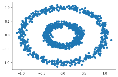
Let’s compare Spectral Clustering to K-means Clustering on a 2 disk pattern.
# make the data
n = 1000
X, y = datasets.make_circles(n_samples=n, shuffle=True, noise=0.05, random_state=None, factor = 0.4)
plt.scatter(X[:,0], X[:,1])
# perfrom k-means clustering
km = KMeans(n_clusters = 2)
km.fit(X)
plt.scatter(X[:,0], X[:,1], c = km.predict(X))
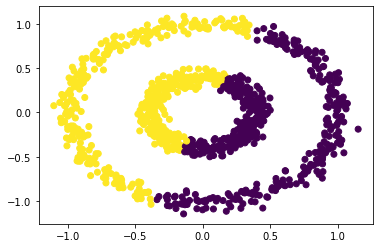
Hmm, not quite right. Let’s try to use spectral_clustering() with epsilon = 0.7.
plt.scatter(X[:,0], X[:,1], c = spectral_clustering(X, 0.7))
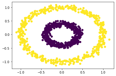
Awesome! Our Spectral Clustering does much better than K-means Clustering on more ‘weird’ data.
But, there is a catch: spectral clustering does not perfectly cluster this data for all values of epsilon.
Let’s see the case of epsilon = 0.1:
plt.scatter(X[:,0], X[:,1], c = spectral_clustering(X, 0.1))
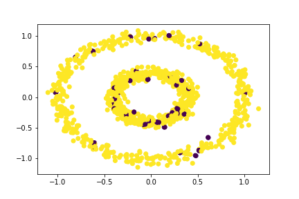
That’s terrible!
Thus, spectral clustering is incredibly effective but only for specific values of
epsilon.