Fake News Prediction with TensorFlow

In this blog post we will use TensorFlow, an open source platform for machine learning to predict fake news from a labeled dataset of news items.
§ Importing the Data
First, let’s import some basic packages.
# import packages
import pandas as pd
import numpy as np
from matplotlib import pyplot as plt
# import the data from a url
url = "https://github.com/PhilChodrow/PIC16b/blob/master/datasets/fake_news_train.csv?raw=true"
data = pd.read_csv(url)
data.head()
-
title: the title of the news item -
text: the text of the news item -
fake: the label for fake (1)/no fake (0) -
Unnamed:0: we can discard this column as it is redundant
| Unnamed: 0 | title | text | fake | |
|---|---|---|---|---|
| 0 | 17366 | Merkel: Strong result for Austria's FPO 'big c... | German Chancellor Angela Merkel said on Monday... | 0 |
| 1 | 5634 | Trump says Pence will lead voter fraud panel | WEST PALM BEACH, Fla.President Donald Trump sa... | 0 |
| 2 | 17487 | JUST IN: SUSPECTED LEAKER and “Close Confidant... | On December 5, 2017, Circa s Sara Carter warne... | 1 |
| 3 | 12217 | Thyssenkrupp has offered help to Argentina ove... | Germany s Thyssenkrupp, has offered assistance... | 0 |
| 4 | 5535 | Trump say appeals court decision on travel ban... | President Donald Trump on Thursday called the ... | 0 |
§ Splitting Data into Training & Test Sets
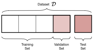
-
Training Data: This dataset consists of
X_train,y_trainwhich contain the features and the output (fake column in our case) respectively. This data will be used to train our model. -
Validation Data: This dataset consists of
X_val,y_valwhich contain the features and the output respectively. After training our model multiple times (or epochs) on the training data, we obtain the values of the optimized parameters. Testing our model on the validation data gives us an idea of the performance of the model on unseen data (testing data). -
Test Data: Using this data is the final stage of the ML pipeline. It is used to measure the model’s performance on unseen data and ultimately the model’s success in achieving the objective of the project.
We will create the training and validation from our main dataset and obtain the testing data from another url at last stage of our modeling process.
# import the package for splitting data
from sklearn.model_selection import train_test_split
x = data[["title","text"]] # the predictor columns
y = data[["fake"]] # the response column
x_train, x_val, y_train, y_val = train_test_split(x,y, random_state = 10, test_size = 0.2) # make the datasets
The training data constitutes 80% of the news items and validation the other 20%
print(x_train.shape, y_train.shape, x_val.shape, y_val.shape)
(17959, 2) (17959, 1) (4490, 2) (4490, 1)
§ Making a TensorFlow Dataset
Since one of the main objectives of this blog is to use TensorFlow for building the model pipeline, we will be using a TensorFlow Dataset instead of a pandas dataset that we currently have.
TensorFlow Dataset objects allow us to design efficient data pipelines with significant less effort.
We need to create new datasets for our training and testing data using tf.data.Dataset which will have a tuple containing 2 dictionaries, for the predictors and response variable respectively:
- A dictionary containing the input columns
textandtitle - A dictionary containing the output column
fake
Let’s begin.
# import these packages
import tensorflow as tf
import nltk
from nltk.tokenize import RegexpTokenizer # will help to remove the punctuation, other special chars and split the string
from sklearn.feature_extraction import text
tensorflow: the main TensorFlow librarynltk.tokenize: helps to remove punctuation from textsklearn.feature_extraction: get the list of redundant words (stopwords)
We will use a function make_dataset to create a TensorFlow Dataset object.
def make_dataset(x,y, stop, batch = 100):
"""
PURPOSE
-----
This function removes stopwords, punctuation, and other characters from
text and title columns of the dataframe.
INPUT
-----
x : a pandas dataframe containing text and title columns
y : a pandas dataframe containing the fake column
stop : a list containing the stopwords to remove
batch: specify the size of each batch
OUTPUT
-----
It returns a batched tf.data.Dataset with two inputs and one output: (text,title) and (fake) respectively.
Batching the data is a very efficient way to process large amounts of information.
"""
# make a copy of the df
df = x.copy()
# convert the text in the columns to lowercase
df['text'] = x['text'].str.lower()
df['title'] = x['title'].str.lower()
tokenizer = RegexpTokenizer(r'\w+') # to remove punctuation and other characters
# removing stopwords and punctuation from the text and title column
df['title'].apply(lambda s: ' '.join([word for word in tokenizer.tokenize(s) if word not in stop]))
df['text'].apply(lambda s: ' '.join([word for word in tokenizer.tokenize(s) if word not in stop]))
# making the tf.data.Dataset, a tuple of two dictionaries
data = tf.data.Dataset.from_tensor_slices(
(
{
"text" : df[["text"]],
"title" : df[["title"]]
},
{
"fake" : y["fake"]
}
)
)
return data.batch(batch)
stopwords = text.ENGLISH_STOP_WORDS # the stopwords from sklearn
# using make_dataset() on the data
train = make_dataset(x_train, y_train, stopwords)
val = make_dataset(x_val, y_val, stopwords)
§ On to Modeling
We have 3 scenarious to predict whether a news item is either fake or not:
- Use only
titlei.e the article content to predict fakeness - Use only
texti.e the title of the article to predict fakeness - Use both
textandtitleto predict fakeness
Let’s make a Neural Network for each of the 3 scenarios and see which one performs the best on the validation data.
Model 1: Using
titleto Predict Fake News
Step 1: Vectorize the title Column
# import these packages
from tensorflow import keras
from tensorflow.keras import layers
from tensorflow.keras.layers.experimental.preprocessing import TextVectorization
from tensorflow.keras import losses
keras: library for Neural Networkskeras.layers: helps create layers for the Neural NetworkTextVectorization: helps vectorize text data into integerskeras.losses: gives options for various loss functions
A neural network cannot understand text, well atleast not in the form of alphabets. We need to transform the text in our input into integer vector representation.
One of the ways to do this is to make a frequency rank matrix in which each entry \(a_{ij}\) represents the rank of the word j in among all articles in terms of frequency, for article i.
Example: If one article title is “Studio Ghibli is best anime” Then it’s rank frequency vector can look like:
[1500,1900,1,50,300]
which means ‘Studio’ is the 1500th most common word in our article corpus, ‘Ghibli’ is the 1900th most common and so on.
Let’s vectorize the text data.
# vectorizing the title column
def create_vectorized_layer(train, feature, size_vocab, output_seq = 500):
"""
PURPOSE
-----
This function creates a TextVectorization object which when applied to text data, converts the text to a frequency rank matrix.
INPUT
-----
train : the data to make the object on
feature: the text feature of the data to make the object on
size_vocab: number of top words to choose
output_seq:
OUTPUT
-----
vectorize_laye: vectorizes input text
"""
# create a TextVectorization object
vectorize_layer = TextVectorization(max_tokens = size_vocab,
output_mode = 'int',
output_sequence_length = output_seq)
vectorize_layer.adapt(train.map(lambda x,y: x[feature])) # learn the top 2000 words
# return the vectorize layer object of the specific input feature in the data
return vectorize_layer
Before we decide how many words to use for size_vocab, let’s look at the total number of unique words (excluding stopwords) in our data.
import itertools
l = []
new = []
stop = text.ENGLISH_STOP_WORDS
tokenizer = RegexpTokenizer(r'\w+')
data['title'].apply(lambda s: l.append(' '.join([word for word in tokenizer.tokenize(s) if word not in stop])))
x = [new.append(words.split()) for words in l]
unique_words = list(itertools.chain(*new))
len(set(unique_words))
26027
We have 26027 unique words. Let’s consider the top 2000 (~7%) words for our model i.e. the top 2000 words according to frequency of occurence in the titles of the articles.
# creating vectorizer for title
vectorize_title = create_vectorized_layer(train, 'title', 2000)
vectorize_title
<tensorflow.python.keras.layers.preprocessing.text_vectorization.TextVectorization at 0x7f38e6ade350>
We will use vectorize_title later to vectorize the title column of the data.
Step 2: Create the Input
We have one input, i.e. title, so we will create a keras.Input object for the same.
# create the title input
title_input = keras.Input(
shape = (1,),
name = "title",
dtype = "string"
)
Step 3: Design the Model
Let’s design the layers of our deep neural network:
# Let's make a function to create the layers of a NN using a single predictor
def make_layers_one(input_var, vocab_size = 2000, embed_size = 5):
'''
PURPOSE
-----
This function makes the layers of a model which uses a single predictor variable
INPUT
-----
input_var: the Keras Input Object of the predictor variable - text/title
vocab_size: the number of initial features as input
embed_size: the dimension of the word embeddings
OUTPUT
-----
returns the layers excluding the output layer
'''
vectorize_var = create_vectorized_layer(train, input_var.name, vocab_size)
features = vectorize_var(input_var)
# creating the layers of the neural network
features = layers.Embedding(vocab_size, embed_size, name = 'embedding_' + input_var.name)(features)
features = layers.Dropout(0.25)(features)
features = layers.GlobalAveragePooling1D()(features)
features = layers.Dropout(0.25)(features)
features = layers.Dense(50, activation='sigmoid')(features)
features = layers.Dense(50, activation='sigmoid')(features)
return features
def make_model(input):
"""
PURPOSE
-----
This funtion creates a Keras model for each of the following scenarios:
1. When input is title
2. When input is text
3. When input is both text and title
INPUT
-----
input: a list of Keras Inputs eg. [title_input]
OUTPUT
-----
model: a neural network ready to train
"""
# Model layers for ONLY input
if (len(input) == 1):
all_layers = make_layers_one(input[0])
output = layers.Dense(2, name = "fake")(all_layers) # the output layer
# Model layers for both title and text input
if len(input) == 2:
layers_first_var = make_layers_one(input[0]) # layers for variable 1
layers_second_var = make_layers_one(input[1]) # layers for variable 2
main = layers.concatenate([layers_first_var, layers_second_var], axis = 1) # combine the above layers
main = layers.Dense(50, activation = 'sigmoid')(main) # add another layer
output = layers.Dense(2, name = "fake")(main) # final output layer
# create a model object
model = keras.Model(
inputs = input,
outputs = output
)
# specify the optimization method and the type of loss function to minimize
model.compile(optimizer = "adam",
loss = losses.SparseCategoricalCrossentropy(from_logits=True),
metrics=['accuracy']
)
return model
We have constructed the skeleton of our model; all it’s missing is the data to be fed into it. Let’s see the skeleton of the model:
model = make_model([title_input])
model.summary()
Model: "model"
_________________________________________________________________
Layer (type) Output Shape Param #
=================================================================
title (InputLayer) [(None, 1)] 0
_________________________________________________________________
text_vectorization_1 (TextVe (None, 500) 0
_________________________________________________________________
embedding (Embedding) (None, 500, 5) 10000
_________________________________________________________________
dropout (Dropout) (None, 500, 5) 0
_________________________________________________________________
global_average_pooling1d (Gl (None, 5) 0
_________________________________________________________________
dropout_1 (Dropout) (None, 5) 0
_________________________________________________________________
dense (Dense) (None, 50) 300
_________________________________________________________________
dense_1 (Dense) (None, 50) 2550
_________________________________________________________________
fake (Dense) (None, 2) 102
=================================================================
Total params: 12,952
Trainable params: 12,952
Non-trainable params: 0
_________________________________________________________________
-
Embedding Layer: This layer assigns ach word its own vector. -
Dropout: Makes certain nodes 0 during training to prevent overfitting. -
Global Average Pooling 1D: This layer downscales the output of the previous layer. -
Dense: The most common layer; contains units/nodes and performs non-linear transformation through activation.
Step 4: Fit & Evaluate Model
Our model has 12,952 parameters to train which means 12,952 partial gradients to calculate and optimize for each epoch. Clearly, the optimization problem is is going to have numerous local minima and look something like this:
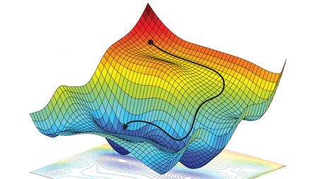
Our starting point in this graph is randomly chosen by the model (the model randomly initializes the parameters for the first layer). Due to hundreds of potential local minima, certain random initializations might give better results at the end of training.
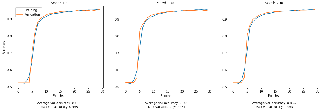
The function below will fit the model for various input seeds:
def run_model(seeds, input, epochs = 30):
"""
PURPOSE
-----
This function fits and evaluates a model, given a list of seeds and input
INPUT
-----
seeds: a list of seed values
input: the input features to train the model on
OUTPUT
-----
figures demonstrating model effectiveness on validation data
"""
fig, ax = plt.subplots(1,len(seeds), figsize = (18,5))
idx = 0
for seed in seeds:
model = make_model(input)
tf.random.set_seed(seed)
history = model.fit(train,
validation_data = val,
epochs = epochs,
verbose = False)
max_accuracy = round(max(history.history["val_accuracy"]),3) # get the max val_accuracy
avg_accuracy = round(np.mean((history.history["val_accuracy"])),3) # get the average val_accuracy
# plot the performance
ax[idx].plot(history.history["accuracy"], label = "Training")
ax[idx].plot(history.history["val_accuracy"], label = "Validation")
ax[idx].set_xlabel(f"Epochs \n\n Average val_accuracy: {avg_accuracy} \n Max val_accuracy: {max_accuracy}")
ax[idx].set_title(f"Seed: {seed}")
ax[0].set_ylabel('Accuracy')
ax[0].legend()
idx += 1
# fitting and evaluating the model
seeds = [10,100,200]
run_model(seeds, input = [title_input] )
Model 2: Using
textto Predict Fake News
Create the Input
# create the text input
text_input = keras.Input(
shape = (1,),
name = "text",
dtype = "string"
)
Design/Create the Model
We will use the same model skeleton that we used above.
model = make_model([text_input])
Fit & Evaluate Model
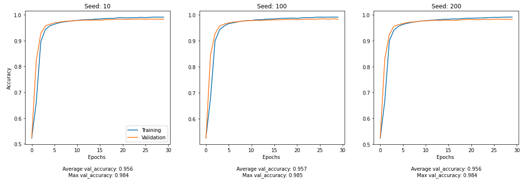
run_model(seeds, input = [text_input])
Model 3: Using both
textandtitleto Predict Fake News
Design/Create the Model
model = make_model([title_input, text_input])
model.summary()
Model: "model_1"
__________________________________________________________________________________________________
Layer (type) Output Shape Param # Connected to
==================================================================================================
title (InputLayer) [(None, 1)] 0
__________________________________________________________________________________________________
text (InputLayer) [(None, 1)] 0
__________________________________________________________________________________________________
text_vectorization_1 (TextVecto (None, 500) 0 title[0][0]
text[0][0]
__________________________________________________________________________________________________
embedding_title (Embedding) (None, 500, 5) 10000 text_vectorization_1[1][0]
__________________________________________________________________________________________________
embedding_text (Embedding) (None, 500, 5) 10000 text_vectorization_1[2][0]
__________________________________________________________________________________________________
dropout_2 (Dropout) (None, 500, 5) 0 embedding_title[0][0]
__________________________________________________________________________________________________
dropout_4 (Dropout) (None, 500, 5) 0 embedding_text[0][0]
__________________________________________________________________________________________________
global_average_pooling1d_1 (Glo (None, 5) 0 dropout_2[0][0]
__________________________________________________________________________________________________
global_average_pooling1d_2 (Glo (None, 5) 0 dropout_4[0][0]
__________________________________________________________________________________________________
dropout_3 (Dropout) (None, 5) 0 global_average_pooling1d_1[0][0]
__________________________________________________________________________________________________
dropout_5 (Dropout) (None, 5) 0 global_average_pooling1d_2[0][0]
__________________________________________________________________________________________________
dense_2 (Dense) (None, 50) 300 dropout_3[0][0]
__________________________________________________________________________________________________
dense_4 (Dense) (None, 50) 300 dropout_5[0][0]
__________________________________________________________________________________________________
dense_3 (Dense) (None, 50) 2550 dense_2[0][0]
__________________________________________________________________________________________________
dense_5 (Dense) (None, 50) 2550 dense_4[0][0]
__________________________________________________________________________________________________
concatenate (Concatenate) (None, 100) 0 dense_3[0][0]
dense_5[0][0]
__________________________________________________________________________________________________
dense_6 (Dense) (None, 50) 5050 concatenate[0][0]
__________________________________________________________________________________________________
fake (Dense) (None, 2) 102 dense_6[0][0]
==================================================================================================
Total params: 30,852
Trainable params: 30,852
Non-trainable params: 0
__________________________________________________________________________________________________
Fit & Evaluate Model
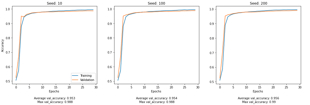
run_model(seeds, input = [title_input, text_input])
§ Which Model Wins?
After analyzing the figures, we can deduce that Model 3 has the highest prediction accuracy on validation data with seed 200!
Let’s see if it is effective on the unseen testing as well.
test_url = "https://github.com/PhilChodrow/PIC16b/blob/master/datasets/fake_news_test.csv?raw=true"
test = pd.read_csv(test_url)
test.head()
| Unnamed: 0 | title | text | fake | |
|---|---|---|---|---|
| 0 | 420 | CNN And MSNBC Destroy Trump, Black Out His Fa... | Donald Trump practically does something to cri... | 1 |
| 1 | 14902 | Exclusive: Kremlin tells companies to deliver ... | The Kremlin wants good news. The Russian lead... | 0 |
| 2 | 322 | Golden State Warriors Coach Just WRECKED Trum... | On Saturday, the man we re forced to call Pre... | 1 |
| 3 | 16108 | Putin opens monument to Stalin's victims, diss... | President Vladimir Putin inaugurated a monumen... | 0 |
| 4 | 10304 | BREAKING: DNC HACKER FIRED For Bank Fraud…Blam... | Apparently breaking the law and scamming the g... | 1 |
# make the tensorflow dataset
x = test[['title', 'text']]
y = test[['fake']]
test = make_dataset(x, y, stopwords)
# evaluate the model on testing data
model.evaluate(test)
225/225 [==============================] - 3s 15ms/step - loss: 0.0504 - accuracy: 0.9845
[0.05042735114693642, 0.984542727470398]
Great! The model predicts unseen fake news items with ~ 98% prediction accuracy.
§ Visualizing Embeddings
Let’s visualize the embeddings we had created in the first layer of our model. These embeddings are words, represented by numeric vectors, that indicate some quality/feature about that word. We will use PCA to reduce the dimension of these embeddings to 2D and 3D in order to visualize them.
weights = model.get_layer('embedding_text').get_weights()[0] # get the weights from the embedding layer
vocab = vectorize_text.get_vocabulary()
A. 3D Visualization
from sklearn.decomposition import PCA
pca = PCA(n_components=3)
weights = pca.fit_transform(weights)
embedding_df = pd.DataFrame({
'word' : vocab,
'X' : weights[:,0],
'Y' : weights[:,1],
'Z' : weights[:,2]
})
embedding_df
| word | X | Y | Z | |
|---|---|---|---|---|
| 0 | 0.064176 | 0.003533 | 0.004457 | |
| 1 | [UNK] | -0.155074 | 0.010242 | -0.017006 |
| 2 | the | -0.192777 | 0.018555 | 0.017560 |
| 3 | to | -1.106134 | -0.028504 | 0.020044 |
| 4 | of | 1.096322 | -0.001871 | 0.012017 |
| ... | ... | ... | ... | ... |
| 1995 | committees | 1.032021 | 0.043653 | 0.013138 |
| 1996 | chuck | 1.593472 | -0.013149 | -0.076570 |
| 1997 | ben | 1.032580 | -0.016551 | -0.038097 |
| 1998 | wearing | -0.711860 | 0.042390 | -0.069730 |
| 1999 | successful | 0.760207 | -0.033267 | 0.090631 |
2000 rows × 4 columns
import plotly.express as px
fig = px.scatter_3d(embedding_df,
x = "X",
y = "Y",
z = "Z",
size = list(np.ones(len(embedding_df))),
size_max = 10,
hover_name = "word",
)
fig.show()
Note: Word embeddings might not appear in Safari (Use Chrome)
2D Visualization
pca = PCA(n_components=2)
weights = pca.fit_transform(weights)
embedding_df = pd.DataFrame({
'word' : vocab,
'X' : weights[:,0],
'Y' : weights[:,1],
})
fig = px.scatter(embedding_df,
x = "X",
y = "Y",
size = list(np.ones(len(embedding_df))),
size_max = 4,
hover_name = "word",
)
fig.show()
